Type of Research Design Observe Then Intervene Then Observe Again

Affiliate 7: Nonexperimental Enquiry

Quasi-Experimental Research

1. Explain what quasi-experimental research is and distinguish it clearly from both experimental and correlational research.
2. Describe three different types of quasi-experimental enquiry designs (nonequivalent groups, pretest-posttest, and interrupted time serial) and identify examples of each one.

The prefix quasi  means "resembling." Thus quasi-experimental research is research that resembles experimental research simply is not true experimental research. Although the independent variable is manipulated, participants are not randomly assigned to conditions or orders of conditions (Cook & Campbell, 1979). ^[one] Because the independent variable is manipulated before the dependent variable is measured, quasi-experimental research eliminates the directionality problem. Only because participants are not randomly assigned—making it likely that there are other differences between conditions—quasi-experimental research does not eliminate the problem of confounding variables. In terms of internal validity, therefore, quasi-experiments are mostly somewhere between correlational studies and true experiments.

Quasi-experiments are nigh likely to be conducted in field settings in which random assignment is difficult or impossible. They are often conducted to evaluate the effectiveness of a treatment—maybe a blazon of psychotherapy or an educational intervention. There are many unlike kinds of quasi-experiments, merely nosotros will discuss simply a few of the near common ones here.

Nonequivalent Groups Design

Call back that when participants in a between-subjects experiment are randomly assigned to atmospheric condition, the resulting groups are likely to be quite similar. In fact, researchers consider them to exist equivalent. When participants are non randomly assigned to conditions, however, the resulting groups are probable to be dissimilar in some ways. For this reason, researchers consider them to be nonequivalent. A , and then, is a betwixt-subjects design in which participants take not been randomly assigned to weather.

Imagine, for case, a researcher who wants to evaluate a new method of pedagogy fractions to third graders. One way would be to conduct a study with a treatment group consisting of i class of 3rd-grade students and a control group consisting of another grade of third-course students. This pattern would exist a nonequivalent groups design because the students are not randomly assigned to classes past the researcher, which means there could be important differences betwixt them. For example, the parents of college achieving or more motivated students might take been more likely to request that their children be assigned to Ms. Williams'south class. Or the principal might have assigned the "troublemakers" to Mr. Jones's form considering he is a stronger disciplinarian. Of grade, the teachers' styles, and even the classroom environments, might exist very unlike and might cause different levels of accomplishment or motivation among the students. If at the stop of the study there was a departure in the two classes' knowledge of fractions, it might have been caused by the deviation between the pedagogy methods—only it might accept been acquired by whatsoever of these confounding variables.

Of course, researchers using a nonequivalent groups design tin can take steps to ensure that their groups are as similar every bit possible. In the present case, the researcher could try to select 2 classes at the aforementioned school, where the students in the two classes have similar scores on a standardized math examination and the teachers are the same sex, are close in age, and accept similar teaching styles. Taking such steps would increase the internal validity of the study considering it would eliminate some of the nigh important confounding variables. But without truthful random consignment of the students to conditions, there remains the possibility of other of import misreckoning variables that the researcher was not able to control.

Pretest-Posttest Blueprint

In a, the dependent variable is measured once before the treatment is implemented and once after it is implemented. Imagine, for case, a researcher who is interested in the effectiveness of an antidrug education program on simple school students' attitudes toward illegal drugs. The researcher could measure the attitudes of students at a item elementary school during one week, implement the antidrug program during the next week, and finally, measure out their attitudes over again the following week. The pretest-posttest blueprint is much like a within-subjects experiment in which each participant is tested showtime under the control status and and so under the treatment condition. It is unlike a within-subjects experiment, withal, in that the social club of atmospheric condition is not balanced because it typically is not possible for a participant to exist tested in the treatment condition starting time and and then in an "untreated" control condition.

If the average posttest score is better than the boilerplate pretest score, and then it makes sense to conclude that the treatment might be responsible for the improvement. Unfortunately, one often cannot conclude this with a high degree of certainty because at that place may be other explanations for why the posttest scores are improve. I category of alternative explanations goes nether the name of. Other things might have happened between the pretest and the posttest. Perhaps an antidrug programme aired on television and many of the students watched it, or perhaps a celebrity died of a drug overdose and many of the students heard about it. Another category of alternative explanations goes under the name of. Participants might have inverse between the pretest and the posttest in means that they were going to anyhow because they are growing and learning. If it were a yearlong program, participants might become less impulsive or meliorate reasoners and this might be responsible for the change.

Some other alternative explanation for a change in the dependent variable in a pretest-posttest design is. This refers to the statistical fact that an individual who scores extremely on a variable on ane occasion will tend to score less extremely on the next occasion. For case, a bowler with a long-term average of 150 who suddenly bowls a 220 will nearly certainly score lower in the next game. Her score will "regress" toward her mean score of 150. Regression to the mean tin be a problem when participants are selected for further studybecause of their extreme scores. Imagine, for example, that only students who scored especially low on a examination of fractions are given a special preparation program and and so retested. Regression to the hateful all but guarantees that their scores will be higher even if the preparation plan has no effect. A closely related concept—and an extremely important one in psychological inquiry—is. This is the trend for many medical and psychological problems to improve over time without whatsoever form of treatment. The common common cold is a good case. If one were to measure symptom severity in 100 common cold sufferers today, give them a basin of craven soup every day, so measure their symptom severity once again in a week, they would probably exist much improved. This does non mean that the chicken soup was responsible for the improvement, notwithstanding, considering they would take been much improved without any treatment at all. The same is truthful of many psychological problems. A group of severely depressed people today is likely to be less depressed on boilerplate in 6 months. In reviewing the results of several studies of treatments for depression, researchers Michael Posternak and Ivan Miller constitute that participants in waitlist control atmospheric condition improved an average of 10 to 15% before they received any treatment at all (Posternak & Miller, 2001)^[2]. Thus ane must generally be very cautious about inferring causality from pretest-posttest designs.

Early studies on the effectiveness of psychotherapy tended to use pretest-posttest designs. In a classic 1952 article, researcher Hans Eysenck summarized the results of 24 such studies showing that about two thirds of patients improved between the pretest and the posttest (Eysenck, 1952) ^[iii]. But Eysenck besides compared these results with archival data from state infirmary and insurance company records showing that similar patients recovered at virtually the same rate without  receiving psychotherapy. This parallel suggested to Eysenck that the improvement that patients showed in the pretest-posttest studies might exist no more than spontaneous remission. Note that Eysenck did non conclude that psychotherapy was ineffective. He simply ended that there was no prove that it was, and he wrote of "the necessity of properly planned and executed experimental studies into this important field" (p. 323). You can read the entire commodity here: Classics in the History of Psychology.

Fortunately, many other researchers took up Eysenck's challenge, and by 1980 hundreds of experiments had been conducted in which participants were randomly assigned to treatment and command conditions, and the results were summarized in a classic book by Mary Lee Smith, Gene Glass, and Thomas Miller (Smith, Glass, & Miller, 1980) ^[4]. They found that overall psychotherapy was quite effective, with about 80% of treatment participants improving more the average control participant. Subsequent research has focused more on the atmospheric condition under which dissimilar types of psychotherapy are more than or less effective.

Interrupted Fourth dimension Series Design

A variant of the pretest-posttest design is the . A time series is a set of measurements taken at intervals over a flow of time. For example, a manufacturing visitor might measure its workers' productivity each week for a year. In an interrupted time series-design, a fourth dimension series like this one is "interrupted" by a treatment. In i classic example, the handling was the reduction of the work shifts in a manufactory from 10 hours to 8 hours (Melt & Campbell, 1979) ^[5]. Because productivity increased rather quickly subsequently the shortening of the work shifts, and considering it remained elevated for many months later, the researcher concluded that the shortening of the shifts acquired the increase in productivity. Notice that the interrupted time-serial blueprint is like a pretest-posttest design in that it includes measurements of the dependent variable both before and afterwards the treatment. Information technology is unlike the pretest-posttest design, all the same, in that it includes multiple pretest and posttest measurements.

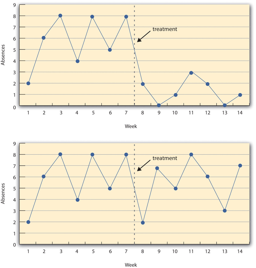
Effigy vii.3 shows information from a hypothetical interrupted time-series study. The dependent variable is the number of educatee absences per calendar week in a research methods grade. The treatment is that the teacher begins publicly taking attendance each twenty-four hour period then that students know that the instructor is aware of who is present and who is absent. The top panel of Effigy seven.3 shows how the data might look if this handling worked. There is a consistently high number of absences before the treatment, and there is an immediate and sustained drop in absences after the treatment. The lesser panel of Figure 7.iii shows how the data might look if this handling did not piece of work. On average, the number of absences after the handling is about the same as the number before. This effigy also illustrates an advantage of the interrupted time-series design over a simpler pretest-posttest design. If there had been just one measurement of absences before the treatment at Week 7 and one afterward at Week viii, then it would accept looked as though the treatment were responsible for the reduction. The multiple measurements both before and after the treatment propose that the reduction between Weeks 7 and 8 is nothing more than than normal week-to-week variation.

Figure 7.3 A Hypothetical Interrupted Time-Serial Design. The peak panel shows information that propose that the treatment acquired a reduction in absences. The bottom console shows data that advise that information technology did not. [Paradigm description]

Combination Designs

A type of quasi-experimental design that is mostly meliorate than either the nonequivalent groups design or the pretest-posttest design is 1 that combines elements of both. There is a treatment group that is given a pretest, receives a treatment, and so is given a posttest. But at the aforementioned time in that location is a control grouping that is given a pretest, does not  receive the handling, and then is given a posttest. The question, and then, is non simply whether participants who receive the handling meliorate but whether they improve more  than participants who exercise non receive the treatment.

Imagine, for example, that students in one school are given a pretest on their attitudes toward drugs, and then are exposed to an antidrug program, and finally are given a posttest. Students in a similar schoolhouse are given the pretest, non exposed to an antidrug plan, and finally are given a posttest. Again, if students in the treatment condition become more negative toward drugs, this change in attitude could be an effect of the treatment, but it could also exist a affair of history or maturation. If it really is an effect of the treatment, so students in the handling condition should get more negative than students in the control condition. Simply if information technology is a affair of history (eastward.g., news of a glory drug overdose) or maturation (e.g., improved reasoning), then students in the two conditions would be likely to evidence like amounts of modify. This type of design does non completely eliminate the possibility of confounding variables, however. Something could occur at one of the schools but not the other (e.chiliad., a pupil drug overdose), so students at the beginning school would be affected past information technology while students at the other schoolhouse would not.

Finally, if participants in this kind of design are randomly assigned to weather condition, it becomes a true experiment rather than a quasi experiment. In fact, it is the kind of experiment that Eysenck chosen for—and that has now been conducted many times—to demonstrate the effectiveness of psychotherapy.

• Quasi-experimental inquiry involves the manipulation of an independent variable without the random assignment of participants to conditions or orders of conditions. Amongst the important types are nonequivalent groups designs, pretest-posttest, and interrupted time-serial designs.
• Quasi-experimental enquiry eliminates the directionality problem because it involves the manipulation of the independent variable. It does non eliminate the problem of confounding variables, nonetheless, because it does not involve random assignment to conditions. For these reasons, quasi-experimental research is generally college in internal validity than correlational studies only lower than true experiments.

1. Practise: Imagine that two professors determine to test the effect of giving daily quizzes on pupil operation in a statistics course. They decide that Professor A volition requite quizzes simply Professor B will not. They will then compare the performance of students in their ii sections on a mutual final exam. Listing five other variables that might differ between the two sections that could bear upon the results.
2. Discussion: Imagine that a group of obese children is recruited for a study in which their weight is measured, and so they participate for 3 months in a program that encourages them to be more agile, and finally their weight is measured once more. Explain how each of the post-obit might affect the results:
   1. regression to the mean
   2. spontaneous remission
   3. history
   4. maturation

Epitome Descriptions

Figure 7.3 epitome description: Two line graphs charting the number of absences per calendar week over fourteen weeks. The first 7 weeks are without treatment and the terminal 7 weeks are with treatment. In the first line graph, there are betwixt 4 to 8 absences each week. After the handling, the absences drop to 0 to 3 each week, which suggests the handling worked. In the second line graph, there is no noticeable modify in the number of absences per week after the handling, which suggests the treatment did not piece of work. [Render to Effigy 7.3]

---

preussfornevenithe.blogspot.com

Source: https://opentextbc.ca/researchmethods/chapter/quasi-experimental-research/

Share this post